Extracting Echelle Spectra
1. Subtract the detector bias and remove the overscan region(s):

A portion of an echelle image of a solar-like star taken by HIRES (an echelle spectrograph installed on one of the Keck telescopes in Hawai'i).

The overscan region of the image is to the right highlighted in orange. This region is where the bias of the detector is measured and plays a similar role to a completely separate bias image that other detectors may use.

The region highlighted here is one that contains a noticeable amount of scattered light. Though not typically a major problem for high signal-to-noise spectra, scattered light may need to be removed from noisier spectra as it can wash out the echelle orders entirely.
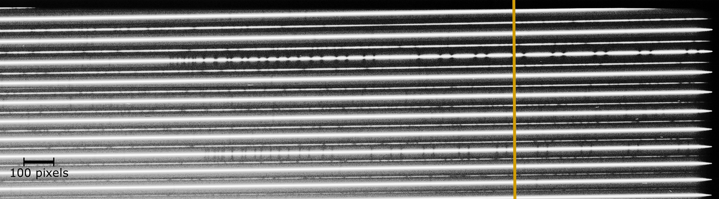
The line drawn here illustrates a cross section of the image along the cross-dispersion direction. A 1D plot of the cross section is shown below.

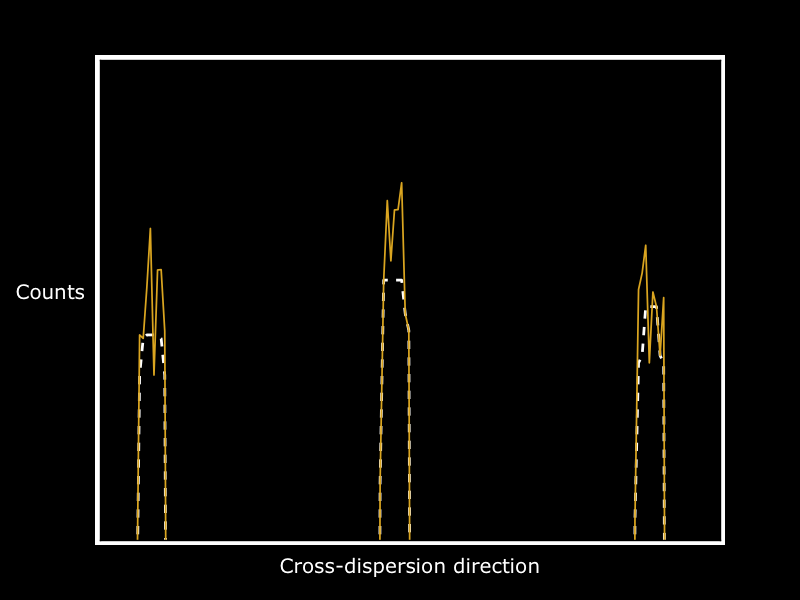
A vertical cross-section of a solar-like star taken by HIRES. Each of the sharp peaks represents an echelle order except for the peak marked by the white dashed line. This dashed line marks a cosmic ray strike. The sky background for one of the orders is highlighted with the white solid line.
2. Create a median-normalized flat field to divide the science spectra by:

A portion of a flat image from HIRES. As above with the science image, a cross section is drawn with this image and shown below.

Like the spectrum of the star above, the flat field image may have a cross section of it plotted in 1D. This is useful in some echelle instruments to quantify the variations in pixel sensitivity.
A vertical cross-section of a flat image taken by HIRES. The orange indicates raw counts and the white dashed line is the median-smooth filter of the counts. This smoothing removes sharp features and provides a comparison to the raw counts to allow the sensitivity of each pixel to light to be measured. By dividing the counts by the median-smooth, each pixel has a value of approximately 1 count and any deviation from 1 count thus quantifies that pixel's sensitivity. This resulting median-normalized image is divided out from the science images.
3. Use a bright star or the daytime sky to define a trace function for each echelle order and use the trace function of each order to extract a spectrum:

A full view of the trace function of a single order from an image from MINERVA. The trace function (see below, right image) for each order is aligned with the trace functions in other images taken the simultaneously (in the same observing night). This alignment allows for a simple integration or optimal extraction over the science image, which may be a lower signal-to-noise ratio than the bright star image.
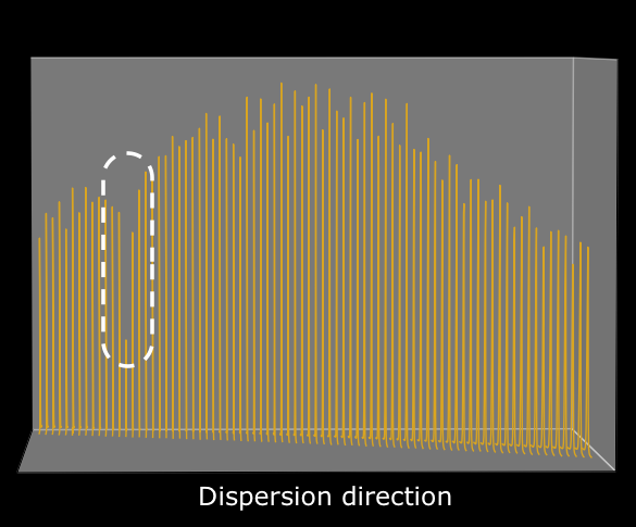
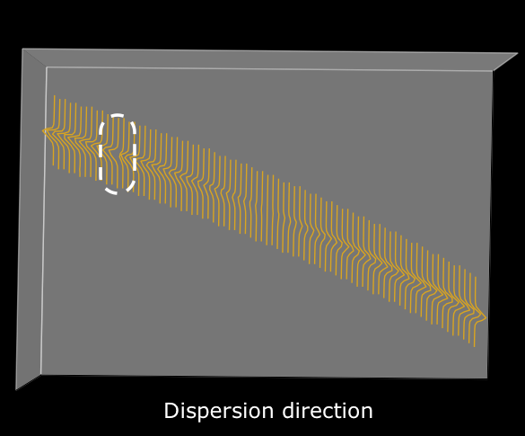
Left image: A view of the above image from the point of view of the dispersion direction of the echelle order. The white dashed line highlights an absorption feature.
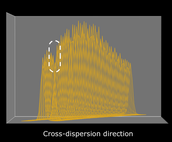
Center image: A view of the above image from the point of view of the cross-dispersion direction of the echelle order. The white dashed line highlights an absorption feature.
Right image: A view of the above image from the point of view of the trace function (a top-down view) of the echelle order. The white dashed line highlights an absorption feature.
4. Fit a function to the detector blaze and divide it out:

An extracted order from the HIRES detector. The white is a rough blaze function polynomial that fits to the top of the data.

A high order polynomial fit to the blaze of a flat field echelle order at best typically results in this plot. The imperfect blaze function fit results in artificial features in the normalized echelle order, which can mimic astrophysical effects.

An improved blaze function fit results in this plot where the location of continuum is clear and there are little to no artificial features introduced by dividing the blaze function out.
5. Use a Thorium-Argon (or other well-known element(s)) spectrum to determine a wavelength solution:
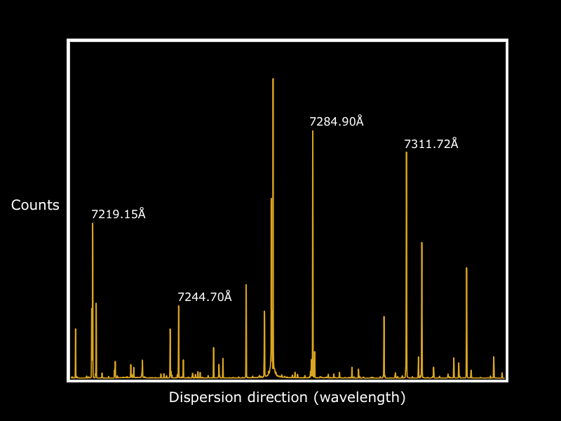
An extracted order from a Thorium-Argon (ThAr) spectrum taken by HIRES. A line list of ThAr needs to be obtained and the line centers (several labelled here), at the moment, need to be compared by hand to the line list.
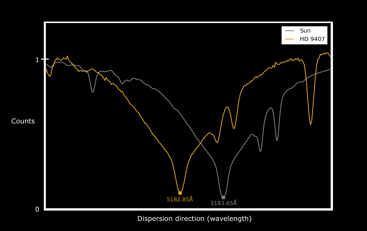
A comparison of HD 9407 to the solar spectrum around one of the magnesium triplet absorption features.
If issues arise during in the reduction pipeline, see the debugging page: